Worst First
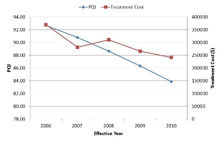
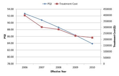
The Worst-First analysis procedure represents the simplest analysis scenario where the user would be interested in addressing the maintenance and repair (M&R) needs of the highway network that rank lowest in terms of a certain performance index. The analysis procedure would progressively address the highway sections that are structurally most deficient until the maintenance budget is exhausted. Thus in essence, this analysis procedure does not involve any optimization as the projects that are selected for receiving M&R treatments are pre-selected. The decision variable selected in the objective function will determine the ordered list of structurally deficient sections and will be sequentially processed subject to the constraints.
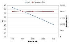
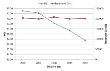
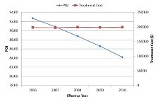
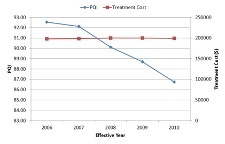
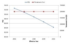
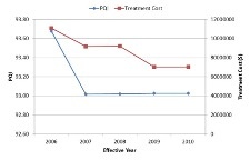
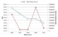
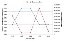
Below, you can see the network level performance indices for two separate scenarios – the first uses Pavement Quality Index (PQI) to define the worst-performing sections while the other uses remaining service life (RSL) to define the same. In either scenario, the maintenance budget was capped at $200,000 and therefore the analysis would terminate when the financial resources are exhausted. It should be noted in this context that the system opts to fund a particular project even when there is available budget to cover half of the project cost as it is reasonable to seek additional resources than underutilizing available funds.
| Worst defined by lowest PQI | Worst defined by lowest RSL |
Prioritization
The Prioritization analysis mechanism is similar to the “worst-case” scenario, though it offers more flexibility for defining the ordered list of highway sections that should take precedence while finalizing the M&R work plan. In the case of “Prioritization”, the priority groovy sets the hierarchy of highway projects and serves as the primary mechanism to define the list of projects that should be shortlisted for the proposed analysis period. In the event where the prioritization is based on the same PI as one would select for a worst-first scenario, they would result in identical scenarios which would lead to identical treatment strategies. However, if the prioritization is based on some other algorithms, the “objective function” in optimization will have no effects on the results because the work plan result is fully determined by the priority value calculated for each section.
However, the priority groovy offers the user with the capability to develop customized scenarios depending on the user’s needs. For example, the agency might be more interested in addressing the M&R needs of the arterial system more than collectors or local residential streets. The priority groovy is useful in such scenarios as it lets the user define the ordered list of highway sections and their relative precedence to receive M&R treatments. However, barring the aforementioned feature, a prioritization analysis is identical to the worst-first scenario as highway sections are selected for M&R activities until the maintenance budget is exhausted. It is also evident that the prioritization analysis procedure does not involve any optimization as the selection of sections is based on the relative ordering of highway sections defined by the priority groovy and therefore the objective function is redundant.
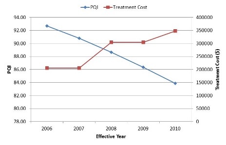
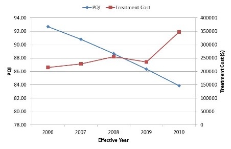
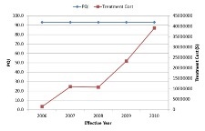
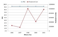
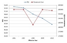
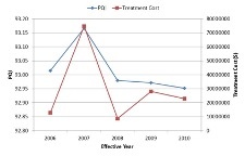
The graphs below demonstrate the network condition for two prioritization analysis scenarios – one based on PQI and the other based on PQI and functional class. While in the first case the treatment selection is finalized based on PQI, the second scenario will give higher preference to projects for higher functional classes.
| Prioritization based on PQI | Prioritization based on PQI & Functional Class |
In Prioritization analysis, a Groovy script is used to calculate the priority value in order to rank projects. The following figure shows the window to configure the groovy script for analysis priority.
Ranking
The Ranking analysis procedure available through the network optimization tool in the PMS module utilizes a benefit-cost approach in finalizing the list of sections that are shortlisted for M&R treatments. In principle, projects are selected in a decreasing order of benefit-cost ratio. Thus, given the analysis procedure, it is essential that the constraint or the objective involves a cost parameter which for most practical purposes would involve the treatment cost. It is essential that the problem includes one and only one constraint. The other half of the problem which involve the benefits that are derived from a certain project can include improvement in PI values or the remaining service life (RSL) for a given highway facility. The overall merit of the specific project will depend on the ratio of the benefit to the incurred cost. A project that offers higher benefits for a relatively low treatment cost will be ranked higher than one that offers relatively low benefits for the same amount of resources expended.
The general procedure of using cost/benefit ranking for project selection is as follows:
- Start with a decision process that gives you an appropriate treatment for each section analyzed.
- Then compute the total benefit and cost for each project.
- Start with the highest benefit to cost ratio project that fits within the budget and select projects in benefit/cost ratio order until the budget is expended.
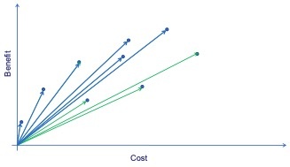
This procedure can be represented graphically as shown in the first figure below. This analysis starts by plotting the alternatives on a benefit cost graph. Each dot represents a possible project. Then the benefit cost ratios for each project are calculated. These are essentially the slope of the lines connecting the origin to the point representing each project. Next, projects are selected based on the highest benefit cost ratio until the budget is exhausted.
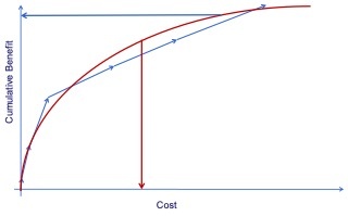
If we plot the cumulative benefit vs. cumulative cost, we get the characteristic shape of the “efficient frontier”, as shown in the second figure below. This is a curve that defines the best decision possible. On the bottom-left part of the curve are the projects with high cost/benefit ratio, indicating a high returns, whereas the top-right part of the curve represents the projects with low cost/benefit ratio, indicating a diminishing returns. Therefore, the curve also shows many features that are intuitive about selecting alternatives. For example, given an allowed budget, we can find the most
| Graphical Representation of Cost/Benefit Ranking Method | The Efficient Frontier |
The graphs below illustrate the ranking analysis through a couple of analysis scenarios where the user may be interested in maximizing the network condition subject to fixed budget or the inverse problem. Furthermore, there might be occasions where the agency might have an existing work plan that needs to be accounted for in determining the treatment options for the entire network. In such scenarios, the network condition has to be updated prior to determination of the provisional work plan.
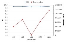
| Ranking – Maximize PQI s.t. Fixed Treatment Cost (w/o WP) | Ranking – Maximize PQI s.t. Fixed Treatment Cost (w/WP) |
| Ranking – Minimize Treatment Cost s.t. Fixed PQI (w/o WP) | Ranking – Maximize PQI s.t. Fixed PQI (w/WP) |
It should be emphasized that the results from cost/benefit ratio ranking are only “near optimal,” meaning there are some situations where this method will “miss” the true optimal results, especially when the scope of an analysis is very small. If there are thousands of projects to choose from, the effect of this problem is very small. However, the cost/benefit ratio ranking method is still worth mentioning because it is a simple method (you can manually perform this analysis in a spreadsheet) that can produce a near optimal results, compared to the method described in the next section, “Multi-Constraint Analysis”, which gives a true optimal result, but requires computerized solver to implement.
Multi-Constraint
The Multi-Constraint Analysis refers to the most generic problem within the class of optimization problems that are solved discrete in time as part of the network optimization tool in the PMS module. As the title suggests, the problem can be specified to handle multiple constraints. Highway agencies are often faced with the challenge of meeting multiple targets, like maintaining a targeted average PI across the network with no more than a specific number of lane-miles below a certain PI. The aforementioned problem can be formulated with two separate constraints that limit the targeted PI and the percent of the network that must be above the specified threshold. The network optimization feature lets the user specify constraints in one of three different ways:
- The total must not exceed specified targets; mostly used to specify treatment costs.
- The weighted average should be greater/lesser than certain thresholds; used for specifying the targeted PI/RSL/Benefits across the network. The weighted average is calculated based on the analysis weight groovy or the SQL expression (discussed later).
- The percent above threshold specifies the minimum percentage of the network that must meet the targeted PI.
Thus, for the example provided earlier, one would select two constraints, one each of the second and the third type to ensure that the PI across the network meets the specified level with no more than a certain fraction below the minimum acceptable PI. Objective functions are specified the same way as constraints, except that they aren’t assigned any constraint value. Furthermore, the decision to maximize/minimize the objective function is determined by the selection made in the “Objective Direction” in the “Setup PMS Columns” screen. In the event where the “Objective Direction” is not explicitly set by the user, the system seeks to minimize columns that relate to costs and maximize everything else.
Each of the four aforementioned analysis procedures can be solved discrete in time. This means that should a user decide to run the analysis across multiple years, the system would solve the problem once for every single year wherein the solution from the previous year will be brought forward to the current year to determine the network condition. Highway agencies are often faced with budget fluctuations across years and therefore need to plan a priori. The “Propagate Years” feature lets the user set individual constraints for every year included in the analysis period separately, thus adding more flexibility to the analysis procedure. It is important to note that the underlying analysis mechanism hardly changes due to incorporation of this feature as the problem would still be the same with the same set of constraints but different constraint limits for the individual years.
On certain occasions, highway agencies might consider higher PI for arterials and expressways to be considered acceptable compared to local and residential streets due to the obvious reason that these facilities cater to higher traffic volumes. On other occasions, the agency might want to allocate a fixed percentage of its annual maintenance budget for preventive maintenance (PM), rehabilitation and full-depth repair work. In order to tackle these scenarios, the AgileAssets PMS module offers the “Activate Constraint Subdivisions” feature which lets the user enforce additional constraints within a certain genre of constraint. The examples included earlier refer to some of the typical scenarios wherein the user might want to refer to this feature.
The collection of graphs below demonstrates the results for the same scenarios that were earlier executed for ranking using a multi-constraint approach. An optimization problem involving a single constraint is similar to “Ranking” (benefit-cost ratio) and therefore the results illustrated in the collections of graphs above and below resemble each other closely.
| Multi Constraint – Maximize PQI s.t. Fixed Treatment Cost (w/o WP) | Multi Constraint – Maximize PQI s.t. Fixed Treatment Cost (w/WP) |
| Multi Constraint – Minimize Treatment Cost s.t. Fixed PQI (w/o WP) | Multi Constraint – Maximize PQI s.t. Fixed PQI (w/WP) |
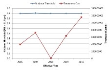
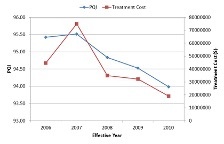
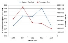
The scenario discussed in the collection of graphs below includes an additional constraint to the aforementioned problem by requiring that 90% of the network has a RSL of 11.5 years. It is understood that the additional constraint will result in higher treatment cost as it has to satisfy additional demands placed on the system. To visualize, the additional constraint adds a new lower bound to the problem which restricts the solution space to fewer choices than that available previously.
Multi-Constraint Analysis – Minimize Cost s.t. PQI >= 93 & % network with RSL = 11.5 yrs >= 90 (w/o WP) |
| |
| Multi-Constraint Analysis – Minimize Cost s.t. PQI >= 93 & % network with RSL = 11.5 yrs >= 90 (w/WP) |
In Treatment optimization analysis, the initial characteristics for all road sections come from the Network Master table. It then uses an integer programming optimization engine to simulate future years. For each year in the analysis period, the following sequence of steps occurs:
- Before the optimization analysis is run, all road sections have their conditions deteriorated by a year.
- Use the decision trees to assign possible treatments.
- The optimization engine is then applied independently of each year of the analysis period.
- At the end of the year, after optimization is run, the road sections that have been rehabilitated have their conditions improved accordingly.
Strategy Analysis
Strategy Analysis refers to a significant shift in the underlying methodology compared to a Multi-Constraint Analysis. The most noticeable difference relates to how the analysis procedure solves the optimization problem across years. In a Multi-Constraint Analysis, the problem is solved discrete in time. This means that the network condition is computed for every single year and treatments are recommended based on the current year’s condition data. The solutions calculated thereof is carried forward to the following year to update the network-level PI and the process is reiterated. With strategy analysis, the network optimization is solved once for the entire analysis period with the objective of determining the optimal solution across the entire planning horizon.
One of the distinguishing features of a strategy analysis is the setup of strategies. A strategy can be defined as a collective treatment plan for a given section over the entire analysis period. As part of the strategy setup, a user would typically specify when he/she anticipates funding to be available with the highway agency to fund any M&R activity for the specific section. Following this step, the system lets the user compute section strategies which involve determination of a possible mix of treatment types over the analysis period, given the available funding sources and the existing network condition. It is important to note that out of all the available treatment strategies, one must include a “No Funding Available” scenario (i.e., Do Nothing) for each of the individual years in the analysis period. This way the user can let the optimization engine determine whether a particular section is in need of any M&R activity at all. The absence of this provision would otherwise force the optimization engine to select a maintenance treatment even when it is not needed. It is also recommended that the user should at least create a few different treatment strategies such that the optimization routine has a sufficient number of feasible solutions for a given section. One should also take into consideration the computation time necessary in the event of an enormously large solution space. Take the example of a user who is working with a network containing tens of thousands of pavement sections and is interested in developing a work plan over a 10-year analysis period. If it is assumed that the user intends to develop strategies for individual sections that are mutually exclusive and exhaustive; the total number of strategies per section would be 210 or 1024 which multiplied by the number of sections leads to more than ten million possible solutions. A problem of this magnitude would require extensive computational effort. It is recommended that engineering judgment should be exercised in developing the treatment strategies to keep the problem manageable.
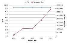
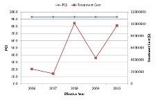
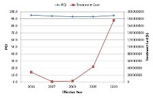
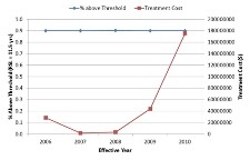
Once the treatment strategies are developed, the subsequent steps are similar to that of Multi-Constraint Analysis wherein the user will need to specify the objective function and the constraints pertinent to the problem. At analysis completion, the proposed work plan will select one of the available strategies for every single section that maximizes/minimizes the objective function subject to the constraints specified. The collection of graphs below demonstrates the results for the same scenarios that were earlier executed for ranking using a strategy approach.
|
| Strategy Analysis – Maximize PQI s.t. Fixed Budget + Minimize Cost .t. PQI = 93 |
|
| Strategy Analysis – Minimize Treatment Cost s.t. PQI = 93 & % Network with RSL >= 11.5 years > 90 |
In short, in Strategy Analysis, for every road section the user will supply several treatment strategies as input. The present value cost and multi-year benefit/condition calculations for each road section and strategy is then used as the input into the integer programming optimization engine. The result is selection of the best life cycle strategy per road section.
The shared components between Treatment and strategy analyses are as follows:
- Use of decision trees (for strategy analyses, it is included in the strategy input phase rather than during analysis). Also, while INCBEN decision trees may be used in strategy analyses, only the first recommended treatment of each decision tree limb will be used and the other two treatment options will be ignored.
- Use of deterioration (but, for strategy analyses, in the strategy input phase rather than during analysis).
- Integer programming engine.
- The same options for objective function and constraints (but, in strategy analyses, applied to the entire rehabilitation life cycle rather a specific rehabilitation recommended for a section in a given year).
The difference between strategy analysis method and Multi-Constraint Analysis include:
- Strategy analysis method optimizes over the entire analysis period rather than a year at a time.
- In order to do that, the input into the integer programming engine is present value costs and multi-year benefit/condition formulations derived from multi-year rehabilitation strategies. These inputs must be pre-calculated.
Strategy Analysis with Work Plan
The strategy analysis discussed in the previous section refers to analysis scenarios that aim to propose a work plan without taking into consideration of any existing work plan. Highway agencies often encounter scenarios where certain projects are shortlisted outside of the purview of the pavement management program. For example, the state department might allocate dedicated funds for improvement of safety standards across the network which might lead to selection of projects that have a history of high accident rates. In other scenarios, certain projects might be included as a result of political intervention or public opinion. For such instances, it would be meaningless to run an analysis that overlooks changes in the network resulting from the existing work plan. The strategy with work plan analysis overcomes this limitation and lets the user include projects from the existing work program. The Strategy with Work Plan analysis is similar to the Strategy analysis. The difference is that the Strategy with Work Plan can include the treatments defined in the master work plan. In Strategy Analysis, even if a MWP is included in the scenario settings, the system will not use it during the analysis. The result of the Strategy with Work Plan type of analysis is the projects and treatments that satisfy the constraints of the analysis.
In the case of strategy analysis, the strategies are computed prior to execution of the optimization routine. The user selects the strategies that he/she wants to associate with a given section and lets the system compute the mix of treatments and the PI for every year included in the analysis period. Thus the optimization routine is not tasked with computation of the network condition at runtime as the PI-s are precalculated. It should be remembered that should a user decide to alter the decision trees or the groovy scripts affecting the RSL calculation or any other instrument that affects the decision variables, the calculated strategies do not apply anymore as they solely relate to the instance that existed prior to the changes made. So one would need to rebuild and re-calculate the strategies anytime changes are made that affect the decision variables. However, in the case of strategy with work plan, the PI across the network is calculated at runtime as the system needs to update the network condition prior to selection of the treatment strategies for a given section. Therefore, running a “strategy with work plan”
scenario without selecting a work plan will be equivalent to the “strategy” scenario except that the strategies will be calculated at run time in the first case but pre-calculated for the latter. It is important to realize that the “strategy with work plan” ensures that the analysis is based on the latest instance of the decision variables and all other instruments that govern them. The fact that the “strategy with work plan” requires computation of PIs, RSL and all other relevant decision variables at run time makes it necessary to design the problem carefully as large networks with hundreds of thousands of sections with an extensive selection of treatment strategies can take several hours of computation time. It is therefore advised that the user should carefully limit the analysis scope to the segment of the network that he/she is interested in determining the maintenance needs. Furthermore, the strategy with work plan offers additional features that allow the user to restrict the scope of the work plan according to his/her needs.
The graphs below demonstrate the results for the same scenarios that were earlier executed for ranking using a Treatment approach.
| Strategy w/WP – Maximize PQI s.t. Fixed Budget | Strategy w/WP – Minimize Cost s.t. PQI ≥ 93 |
| Strategy w/WP – Minimize Cost s.t. PQI ≥ 93 & % of network with RSL ≥ 11.5 years ≥ 90 | |
Estimate MWP Influence
This type of analysis provides the user the ability to determine the network condition if there is already a provisional work plan for the analysis period. The analysis employs deterioration and improvement in the same manner as all other analysis types. The result of this analysis is to show the resultant condition of the network in future years if only the MWP is employed.
This type of analysis type is not to recommend treatment strategies to maintain the network at certain target levels, but only to project the conditions under the selected master work plans. Therefore, there is no requirement for an objective function or constraints to force restrictions on the decision variable. As part of the analysis, the optimization engine takes into consideration the existing work plan and the current network condition. In the following step, the current conditions are updated to reflect the influence of the work plan, carried forward to the following year, and the whole process is reiterated for subsequent years included in the analysis period. The analysis ends with estimates for the network condition and maintenance expenditures, which may be post-processed to generate suitable reports that present the information in a concise format. As in the case of “strategy with work plan”, the user may decide to limit the scope of the analysis to certain routes or functional classes or even restrict the extent of the work plan that is included in the analysis to keep the problem manageable.
