How to Run Optimization Analysis

1.1 General Scenario Setup

In this example, we create and run a multi-constraint optimization network analysis by Perform the following steps: Click Here for Optimization Analysis Exercises

1. Open the Optimization Analysis window: Pavement Analyst > Analysis > Network Analysis > Optimization Analysis.

2. Right-click in the Scenarios pane and then click Insert The system creates a new scenario. An example of the Scenarios pane is shown below.

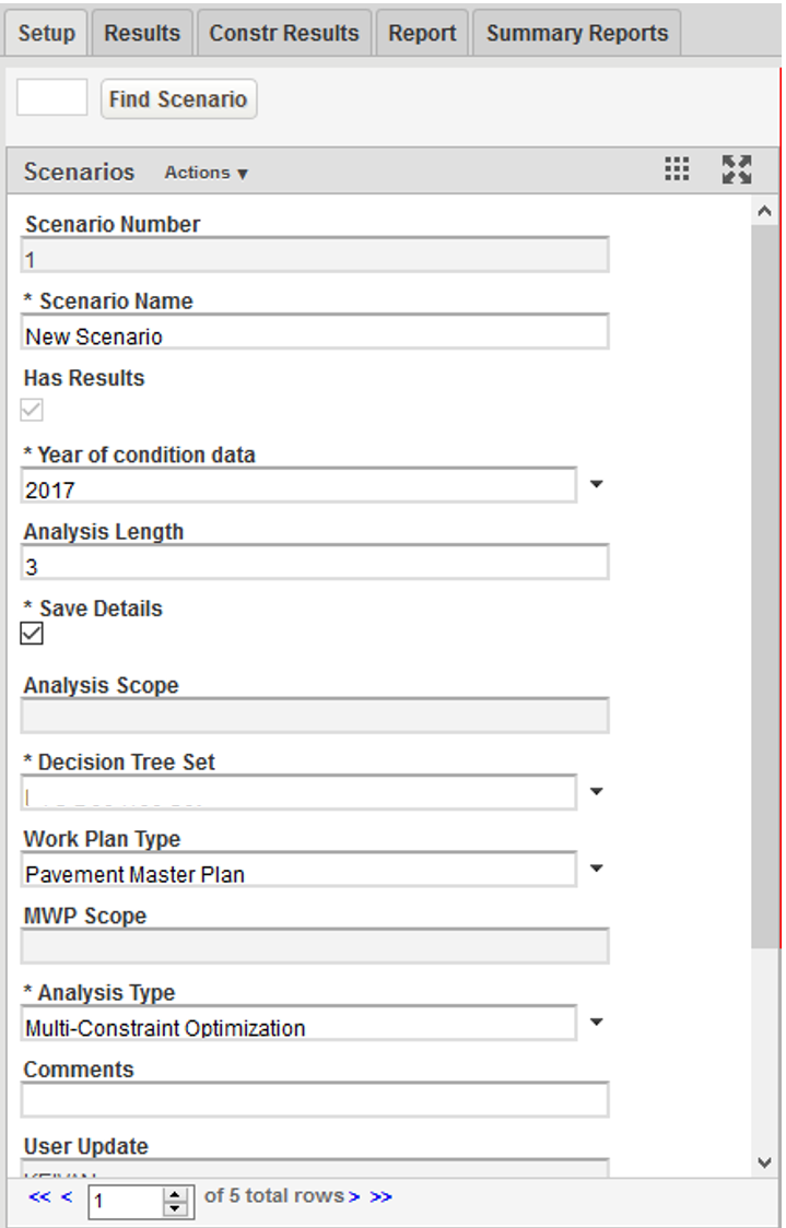
3. Highlight the text in the Scenario Name field and then type the name for this optimization.

4. Click in the Year of Condition data field and select the most recent Network Master data that will be used in the optimization. Note that the year given in this field determines the starting year of the result scenario work plan, which is the entered year plus one.

5. Click in the Analysis Length field and then type the number of years covered by this analysis.

6. If you wish to save the details of the optimization for further study, click the Save Details check box. (The details may be viewed in the Detailed Optimization Results window.)

7. In the Decision Tree Set field, select the appropriate value.

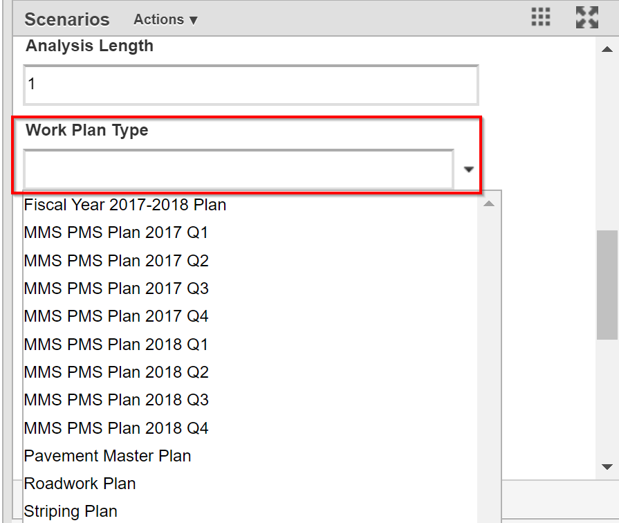
8. If you wish to include a set of master work plan, click the dropdown in the Work Plan Type field and select the desired master work plan type.

9. Click the down arrow in the Analysis Type in the Scenarios pane and then click Multi-Constraint.

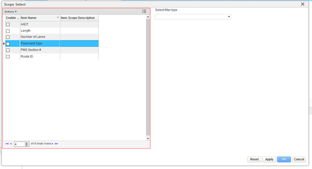
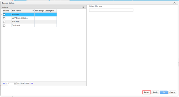
10. If you wish to limit the scope of the network that is used in the analysis, right-click anywhere in this pane and select Edit Scope. This command displays a data selection window that you may use to select what data is used in the analysis.

11. You may restrict the data used from the selected work plan by clicking Edit MWP Scope button. This command displays a dialog box to select what data from the work plan is used in the analysis. An example of this dialog box is shown below.

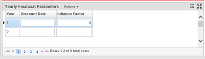
12. If you wish to use a discount rate (that is, the value of money over time) and/or inflation in the analysis, complete the records in the Yearly Financial Parameters pane at the bottom right of the window. Rates are specified in decimal form in this window and can be assigned to all years, or specific years.

1.2 Specify Scenario Objective and Constraints

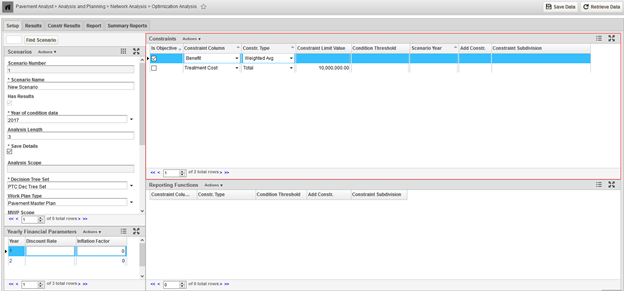
In this example, we enter objectives and constraints in the Constraints pane by performing the following steps: 

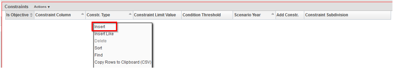
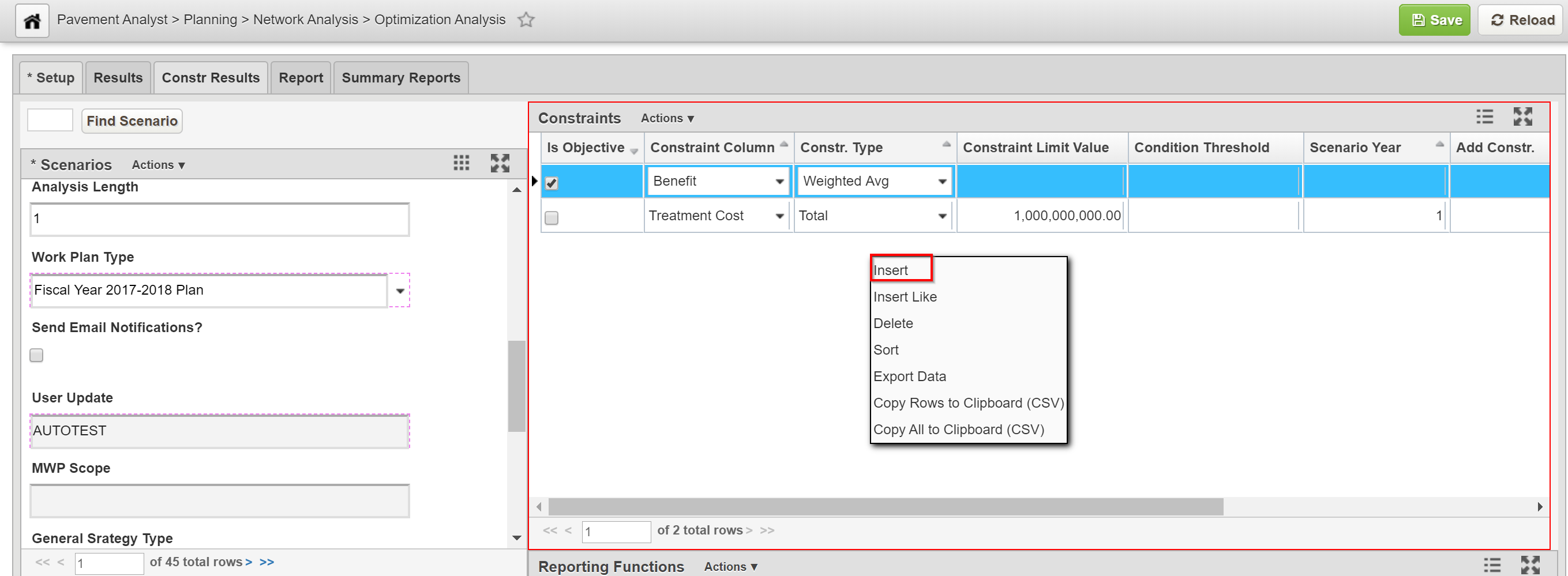
1. In the Constraints pane, right-click anywhere within the table and then click Insert. The system adds a new record to the pane.

2. Click the down arrow in the Constraint Column and then click the desired objective.

3. Click the “Is Objective” check box.

4. Depending on the objective selected, only a certain value may be permitted for the Constr. Type column and so the application automatically sets this column. If this does not occur, click the down arrow in the Type column and then click the appropriate constraint type.

Pavement Analyst supports three types of the Constraints:

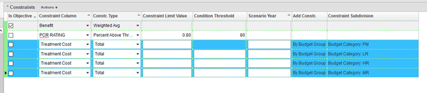
• Total: The analysis engine will use the total amount of the Constraint Column as an objective, or compare it with the value shown in the Constraint Limit Value Treatment Cost is a good example.
• Weighted Average: The analysis engine will use the weighted average value of the Constraint Column as the objective, or compare it with the value shown in the Constraint Limit Value In Pavement Analyst, the weight is set to Lane Miles of each segment. Surface Score is a good example of this constraint type.
• Percent above Threshold: The analysis engine will use the percentage above a particular threshold as the objective, or compare it with the value shown in the Constraint Limit Value The value for the threshold is entered in the Condition Threshold column and the percentage value is entered in the Constraint Limit Value column (in decimals). For example, if you want the lane-miles of Pavement with PCR Rating >=80 to be less than 80%, when translated to this constraint type, this is how to set this constraint

5. While only one objective is allowed for an optimization, one or more constraints may be configured. A constraint record may apply to all years in the optimization period or multiple constraint records may be created for each year in the optimization period.

6. Finally, for those constraints that have subdivisions, you may create records for each constraint subdivision. An example of a Constraint Subdivision would be “Budget Category: MR should not spend more than $2M” or “Interstates should have a minimum weighted Surface Score of 7”, instead of one constraint applying to the entire network. The following steps provide a general process for entering subdivided constraint records.

7. In the Constraints pane, right-click and then click Insert. The system adds a new record to the pane. Do not check the “Is Objective” field.

8. Click the down arrow in the Constraint Column and then click the desired constraint metric.

9. Click the down arrow in the Constr. Type column and then click the desired constraint type.

10. In the Constraint Limit column, enter the value for the constraint.

11. If the constraint type is Percentage Above Threshold, enter the threshold value in the Condition Threshold column.

12. If the constraint applies to all years in the optimization period, leave the Scenario Year field blank. Otherwise, right-click the constraint record and then click Propagate Years in the shortcut menu. The system enters a constraint record for each year in the optimization period as a copy of the record you right-clicked. It also enters the year in the Scenario Year field. You will now need to edit each newly inserted record to reflect the appropriate constraint limit. You can also delete any years where the constraint does not apply.

13. If the constraint will apply to all subdivisions of the constraint (if any), then you are finished with this constraint and may proceed to enter additional constraints as needed. On the other hand, if the constraint limit will vary for the different constraint subdivisions, right-click the constraint record and then click Activate Constraint Subdivisions in the shortcut menu. The system displays a dialog box so you may select a type of constraint subdivision. An example of this dialog box is shown below.

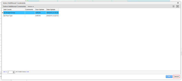
Click the record for the desired type of constraint subdivision and then click the OK button. The system closes the dialog box and inserts a record for each constraint subdivision shown in the Setup Constraint Subdivisions window. The system places the name of the type of constraint subdivision in the Add. Constr. column and the name of the constraint subdivision in the Constraint Subdivision column as shown in the example below.

You now need to edit each newly inserted record to reflect the appropriate constraint limit. After editing each record, you may proceed to enter additional constraints as needed.

1.3 Define Scenario Reporting Function

In this example, we insert a reporting function by performing the following steps:

1. Open the Optimization Analysis window: Pavement Analyst > Analysis > Network Analysis > Optimization Analysis.

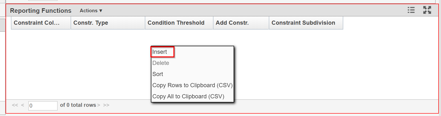
2. Right-click in the Reporting Functions pane and select Insert.

3. Click the Constraint Column drop-down and select the appropriate value.

4. Click the Constr. Type drop-down and select the appropriate value.

5. Click in the Condition Threshold column in type in the numeric value.

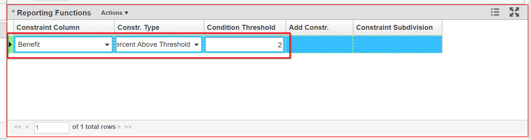
6. Click the Save button to save the record.

1.4 Include Master Work Plan Projects

In this example, we include a project by performing the following steps:

1. Open the Optimization Analysis window: Pavement Analyst > Analysis > Network Analysis > Optimization Analysis

2. In the Scenarios pane, click the Work Plan Type drop-down and select a Work Plan. 

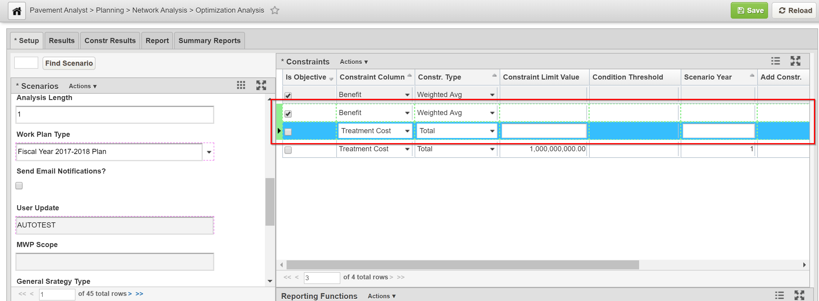
3. In the Constraint pane, right-click and then click Insert. The system adds a new record to the pane.

4. If you haven’t set up the objective, click the down arrow in the Constraint Column column and then select Benefit. You will receive a notification saying “Benefit must have constraint type of ‘Weight Average’”, and the application will select “Weighted Average” for you under Type column. Check the “Is Objective” checkbox at the beginning of this item.

5. Insert another constraint and assign “Treatment Cost” to it. Right click and constraint and select “Propergate Years”. Now this constraint has a line for each year in the analysis period.

6. Right-click on any “Treatment Cost” constraint, and then select Set to Include MWP budget. The application will now calculate the treatment costs for all MWP projects that are within the boundary of the analysis scope.

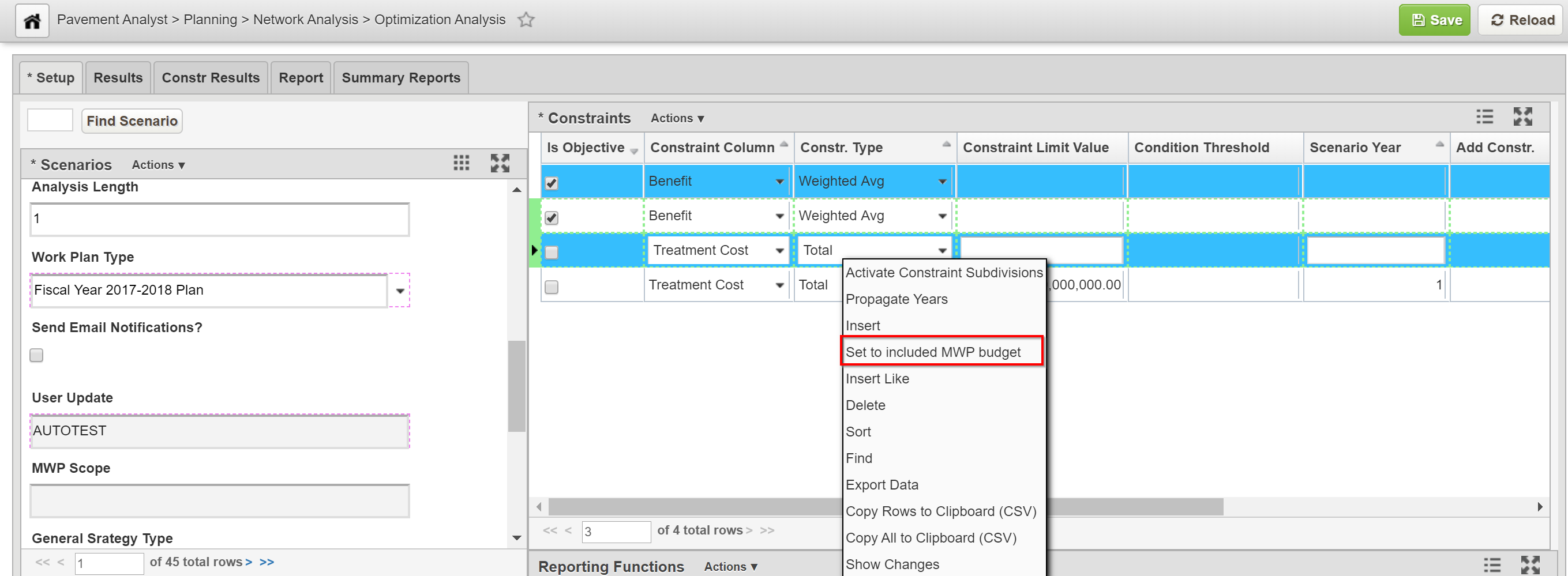
7. When finished, notice the MWP Budget column of the Constraints pane is now populated. This shows how much budget is needed at least to finish the projects in MWP.

8. Examine all Treatment Cost constraints (by Plan Year, Budget Category and Region) and see if they are equal or bigger than MWP Budget. Increase the value where needed to allow for more projects.

1.5 Run Analysis Scenarios

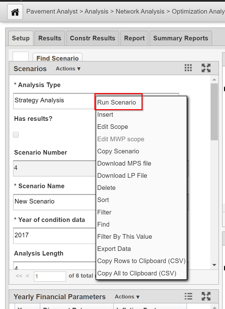
Once all constraints and reporting functions are configured, you are ready to run the optimization. Right-click  in the Scenario pane and select Run Scenario. The application performs the optimization and then displays the results in the Results tab. The Constr. Results tab will also show the actual constraint values at the end of the optimization analysis. You can click the Hide button while performing other tasks. When the scenario is finished, you will receive a notification in the system.

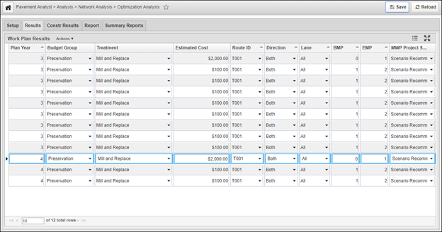
1.5.1 Review Scenario Work Plan Results

The Results tab of the Optimization Analysis window provides a list of work plans produced by the optimization routine, based upon the input criteria configured in the Setup tab. These pavement sections constitute the recommended work plan.

When you right-click this pane, the system displays a shortcut menu. This menu contains Update Cost command that can be used for re-calculating the cost for the selected record.

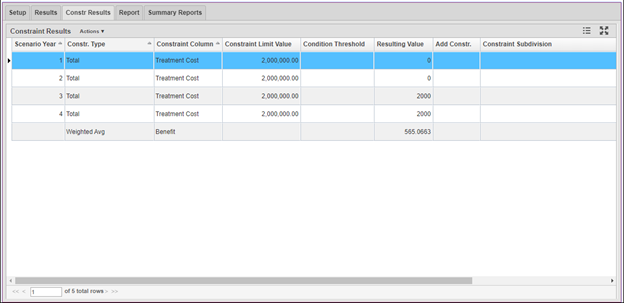
1.5.2 Review Scenario Constraint Results

The Constr. Results tab of the Optimization Analysis window shows the predicted values of each constraint compared to the input constraint value.  This allows you to identify the constraints that have controlled the analysis results.

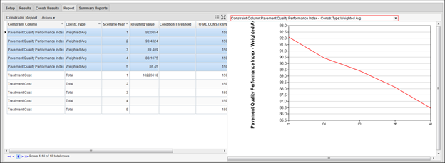
1.5.3 Review Report

The Report tab of the Optimization Analysis window shows the constraints you selected in the Reporting Functions pane of the Setup tab and the values of the constraints.

The right pane shows a graph of the values of a particular constraint (which is selected from the drop-down list field shown at the top of the pane). The Y-axis of the graph shows constraint values and the X-axis shows the number of years in the analysis. The graph is a line graph for all constraint types except Total, which is a bar graph. You may modify the appearance of the graph by using the right-click Change Graph Properties commands.

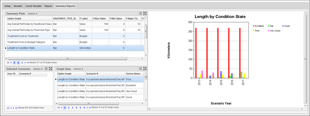
1.5.4  Review Summary Report

Summary Report window displays the summary graphs of each analysis scenario. These graphs are defined in “Setup Graphs for Summary Report” window and will be the same across all analysis scenarios. The x-axis of each graph is the scenario year, whereas y-axis is defined by an SQL expression. Multiple series can be defined for each graph for comparison purpose among different series. For example, a “Length by Condition State” summary report will display the lane-miles of each condition state for each year, where the scenario year is displayed as the x-axis, the total lane-miles is displayed as the y-axis, and Condition State is displayed as different Series. All these parameters can be configured “Setup Graphs for Summary Report” window.

The left top pane shows each type of summary report, the left bottom pane shows the summary data by each series and scenario year, and the right pane displays the summary graph. You may modify the appearance of the graph by using the right-click Change Graph Properties command.

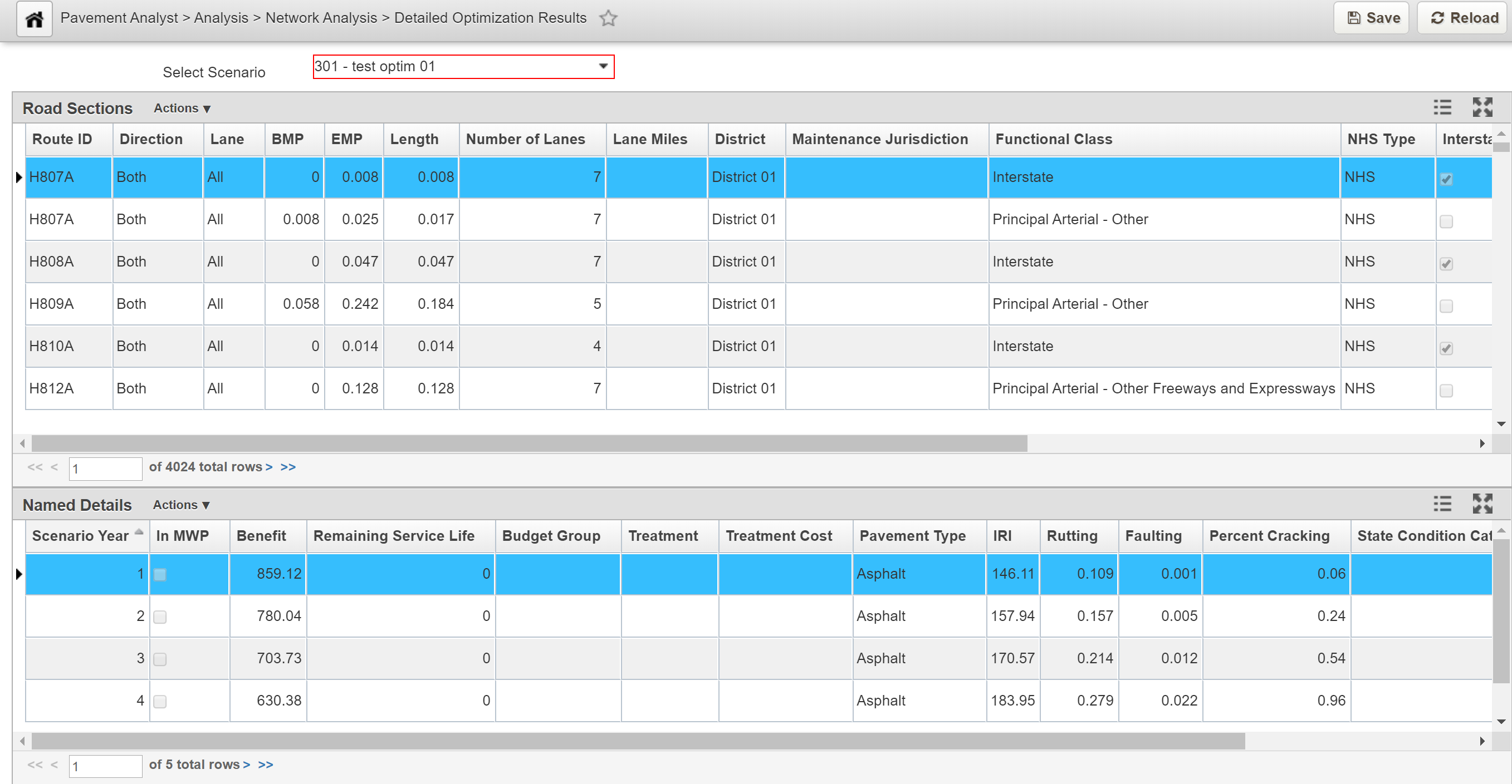
1.6 Detailed Analysis Results

For all analysis scenarios that have the Save Details check box in the Setup tab checked, the Detailed Optimization Results window (s) provides an in-depth look at the data resulting from the optimization. The user can select a desired scenario from the drop-down list in the Select Scenario field at the top of the window, and then the system displays the details data from the scenario.

The upper pane (Road Sections) shows the Network Master sections as defined in the Analysis Scope of the analysis. For the road section selected in the upper pane, the bottom pane (Named Details) shows each year's results for the road section.

LikeBe the first to like this