The Optimization Analysis window is where all optimizations are performed. In this window you can define and run multiple optimizations, each having different settings, budgets, and analysis periods. The results from each optimization are stored separately and can be reviewed in this and other windows throughout the system.

Window Path: Pavement Analyst > Analysis > Network Analysis > Optimization Analysis

The window provides the following tabs that allow you to switch between different components of project optimization

• Setup: This tab is where all parameters for an optimization are established.
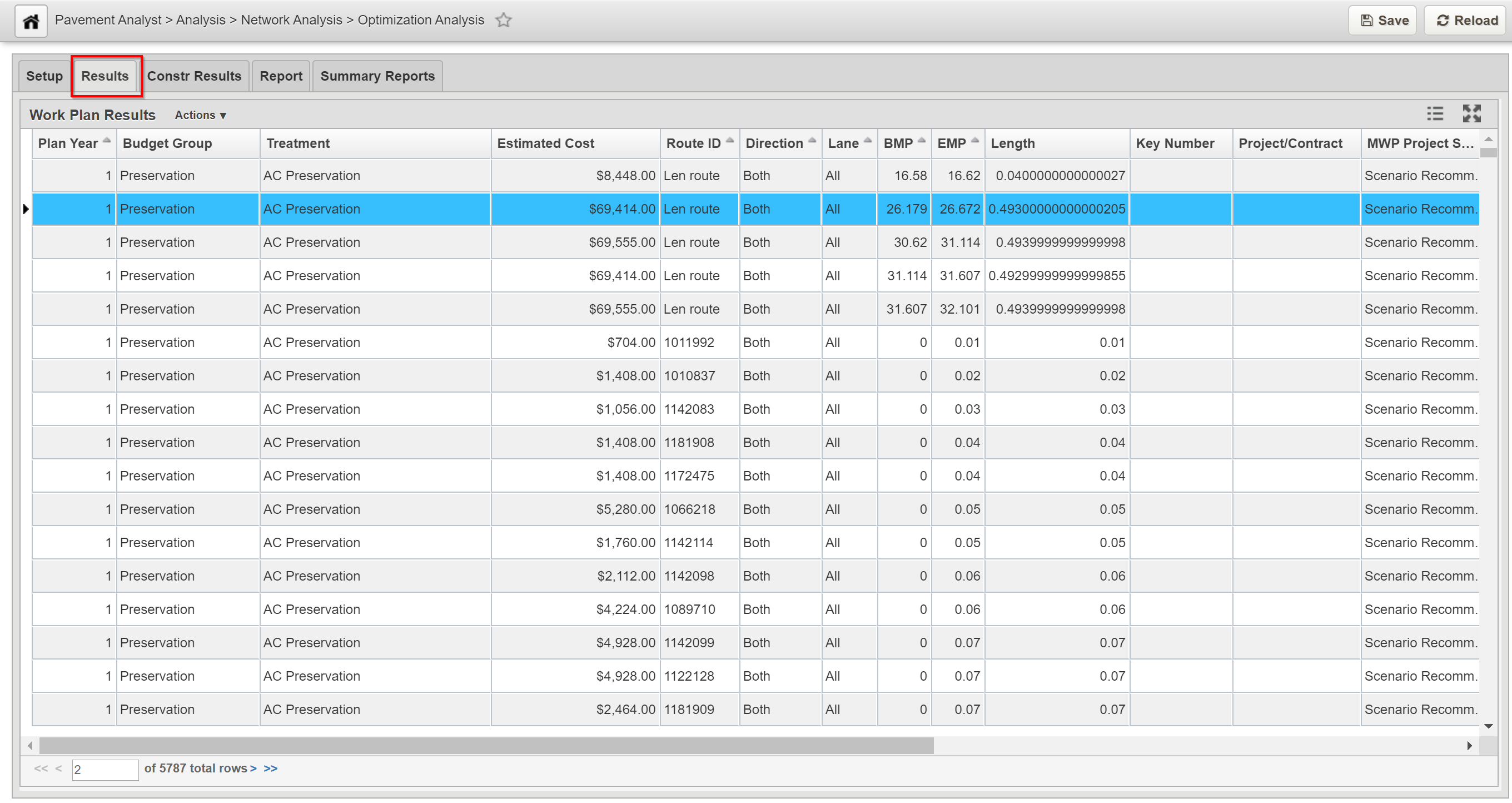
• Results: This tab shows the optimal recommended work plan.
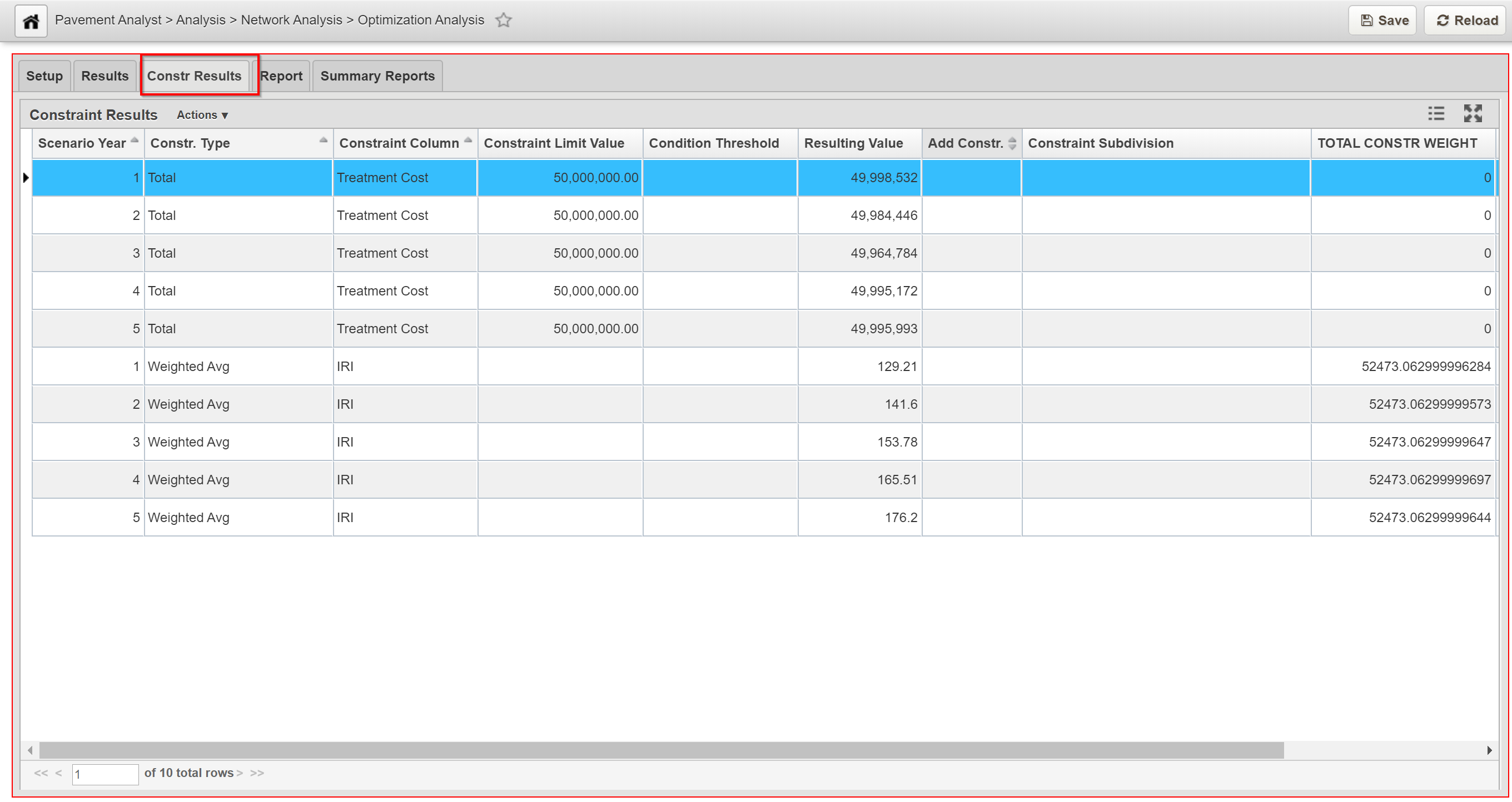
• Constr. Results: This tab shows the predicted values of each constraint compared to the input constraint value. This allows you to identify the constraints that have controlled the analysis results.
• Report: This tab shows the constraints selected in the Reporting Functions pane of the Setup tab and the value of each constraint after optimization
• Summary Report: When an optimization analysis has results, this tab becomes available. It provides a less data-intensive way to view graphs using data from the selected optimization analysis. It also allows you to compare two different optimization analyses.

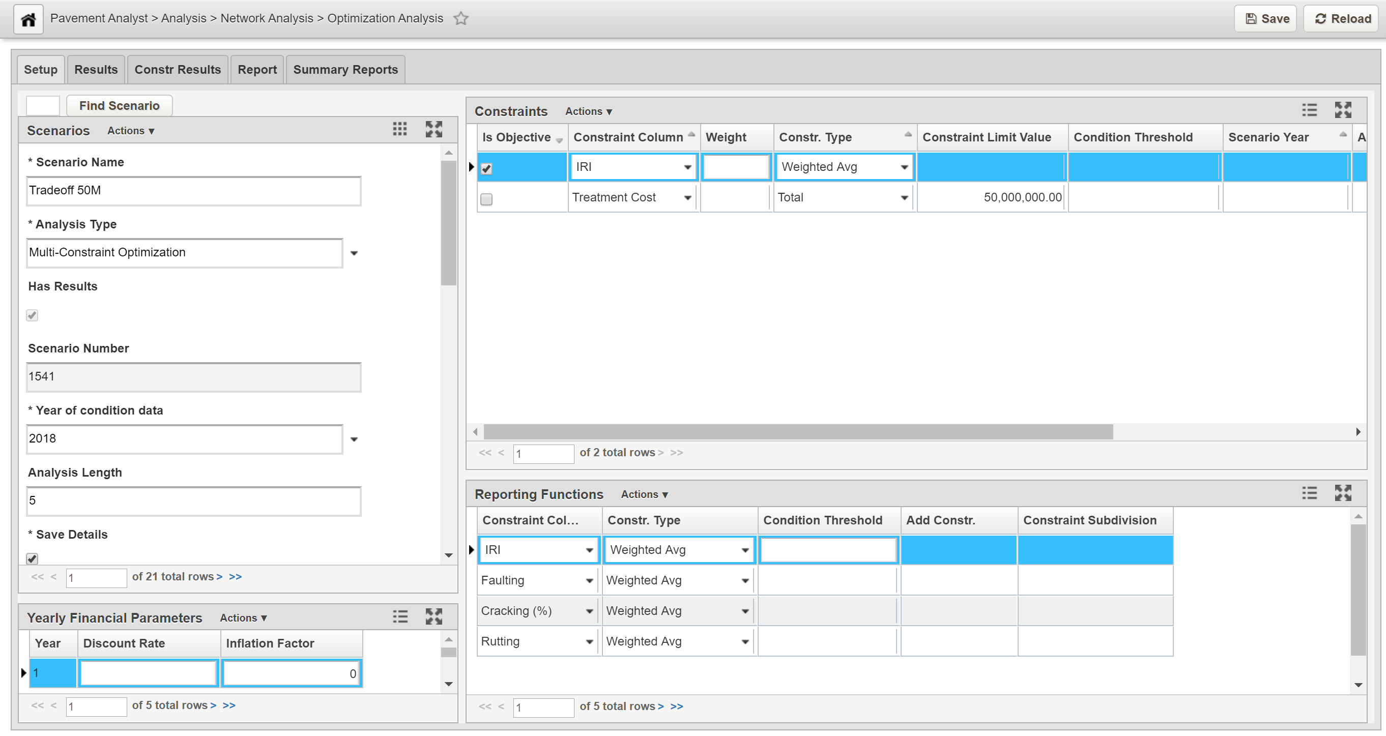
Setup Tab

 This tab contains the Scenarios pane in the upper portion of the window, the Constraints pane on the lower left, a Reporting Functions pane on the lower right and a Yearly Financial Parameters pane on the extreme lower left. 

1.1 Scenarios pane

This pane displays all the analysis scenarios and their parameters. It allows the user to edit the following system configuration-related fields.

Parameters that are displayed in this pane are:

• Analysis Type: This field shows the type of the selected analysis scenario.
• Has Results: This read-only check box indicates if the optimization has already been run. When a check mark is not displayed, then the results information shown in the other tabs is irrelevant.
• Scenario Number: This read-only field displays the Scenario ID in the system. It allows the user to quickly locate a scenario using the “Find Scenario” button.
• Scenario Name: This field displays the name of the selected scenario.
• Year of Condition Data: This field is used as baseline year to convert between scenario year in the analysis period (1, 2, 3, etc.) and Master Work Plan Year (2019, 2020, etc.). In addition, if Network Master has EFF_YEAR field, then this field acts as a filter for Network Master when selecting sections into optimization.
• Analysis Length: This field defines the length of analysis scenario.
• Save Details: This check box determines whether the system saves the details of the optimization. When it is checked, the details from the analysis are saved and may be viewed in the Detailed Optimization Results window. When it is not checked, the details are not saved, although the overall results of the analysis will still be available in the Results tab.
• Analysis Scope: This read-only field shows the data elements that are included in the optimization. The scope is set with the Edit Scope command (right-click and select “Edit Analysis Scope”).
• Administrative Unit: Analysis scenarios can be restricted by administrative unit. This field is included in the Setup tab and shows which unit "owns" the displayed analysis. For example, if the field shows Headquarters, then only users who select the Headquarters administrative unit when logging on may see and run the analysis.
• Decision Tree Set: This field determines what decision tree set will be used in the analysis.
• Work Plan Type: This field provides a drop-down list of all available work plans (which are defined in the Setup Work Plan Type window). When you select a work plan from the drop-down list, the projects and costs from this work plan are first included in the optimization and then remaining rehabilitation recommendations are taken from decision tree results. If you do not select a work plan, then the optimization is run without consideration of a pre-defined work plan; it gets its rehabilitation recommendations entirely from decision tree results. To remove a work plan from the Work Plan Type field so no plan is selected, highlight the displayed work plan and then press the Delete key.
• MWP Scope: This read-only field shows what work plans are included in the optimization. The plans are included by using the Edit MWP Scope command (right-click and select “Edit MWP Scope”).
• Scheduled: When this check box is selected, the system job Run All Scheduled Optimization Scenarios will execute this scenario. This system job allows all scheduled scenarios to run during off-hours to reduce the impact of the optimization analysis on the performance of the system. When several scenarios are scheduled, the system job will execute them sequentially.
• Round Cost: This field causes the system to round the cost of projects to the selected rounding value before submitting the project to the solver engine. The greater the rounding, the faster the solver will converge on a solution.

  
  

  Note:

  The rounded cost will only show up in the Constr. Results tab. The Results tab and Report tab will still display the real un-rounded treatment cost.

• General Strategy Type: The entries that appear in this list are created and maintained in the Setup General Strategy Types window. This column determines what general strategies will be used in Strategy analysis. 
• Disable GEOM Calculation: This parameter can disable the geometry calculation in the analysis results (i.e., Scenario Work Plan and Detailed Analysis Result) for any location records when they are not needed, to improve performance and reduce disk usage. Later, if needed, user can use the right-click command “Calculate Geometry” to re-calculate them.
• Comments: User can include information in this field to describe the optimization.

1.2 Constraints pane

For any analysis type other than “Estimate MWP Influence”, the scenario must have one (or more) objective(s) and constraints.

The system supports three types of constraint/objectives:

• Total: The analysis engine will stop when the constraint reaches the total amount shown in the Constraint Limit Value column. Typically, this type is only used on Treatment Cost to constraint on budget.
• Weighted Average: The analysis engine will constraint the weighted average value of a column using the Index Weight of each segment defined through Calculated Expression window.
• Percent above Threshold: The analysis engine will stop when the constraint value exceeds a threshold value by a certain percentage. The value for the threshold is entered in the Condition Threshold column and the percentage value is entered in the Constraint Limit Value column.

This Constraints pane of Optimization Analysis window contains the following fields:

• Is Objective: A check mark in this column indicates that the selected constraint is the objective of the analysis. You may select more than one objective, but if so the Constr. Type column should be set to Weighted Average, with the objective weights entered in the Objective Coefficients column.
• Objective Coefficient: This column is left blank unless you select multiple objectives. In this case, this column indicates the relative weight of each objective against the others.
• Constraint Column: This column contains a drop-down list. The list contains those columns with a check mark in the Is Constraint check box in the Setup Analysis Columns window. The constraint you select for this column is either the objective of the analysis or acts to limit what is considered for inclusion in the work plan by the analysis engine.
• Type: This column contains a drop-down list of the allowed constraint types: Percent above Threshold, Total, and Weighted Average. 
• Constraint Limit Value: This column is left blank except when the “Is Objective” column is checked for the “Constraint Column”. This column sets the limit value that must be satisfied during analysis. For “Total” constraint type, this column sets a cumulative value that will cause the analysis engine to stop. For “Weighted Average” constraint type, this column sets the lowest or highest value of weighted average of the constraint. For “Percent above Threshold” constraint type, this column sets the threshold value that the constraint value must exceed (by a certain percentage) for the analysis engine to stop. For this type, this column supplies the percentage value that will cause the analysis engine to stop. The percentage value is entered as a decimal value (for example, 10% is entered as 0.1).
• Condition Threshold: This column is left blank except when the Constr. Type column is set to “Percent above Threshold”. This column sets the threshold value for the section condition above which the sections will be counted. For example, if the constraint is “more than 70% of the lane-miles have IRI lower than 2 m/km,” this column will be set to “2”, and Constraint Limit Value column will be set to 0.7.
• Scenario Year: This column is left blank for a constraint if the constraint will apply across all years of the analysis period. If the constraint will vary by year, then fill this field by right-clicking the pane to display the shortcut menu and then click Propagate Years. The system will then create multiple records for the selected constraint, one for each year of the analysis period, and insert the analysis year in this column for each constraint record.
• Add Constr and Constraint Subdivision: These two columns will display the sub-divisions information if this function is activated. When the Activate Constraint subdivision command is executed, the system inserts records for each sub-constraint in the selected constraint subdivision. It enters the name of the constraint subdivision in the Add Constr. column and the name of the sub-constraint in the Constraint Subdivision column.

When right-clicking this pane, the following special commands are available along with the common commands:

• Activate Constraint Subdivisions: This command inserts records for each of the constraint subdivisions into which the selected constraint is subdivided as configured in the Setup Constraint Subdivisions window.
• Propagate Years: This command inserts a record for each of the years in the analysis period that is the same as the record you right-clicked (other than year).
• Set to Included MWP Budget: This command identifies the MWP projects that match the year and constraint partition of the record (and are within the analysis scope and MWP scope). It then calculates a total cost for these identified projects and inserts the cost in the MWP Budget field of the Treatment Cost constraint. 
• Copy MWP Budget to RHS: RHS (Right Hand Side) here means the constraint limit value for Treatment Cost constraint. This command copies the value in “MWP Budget” field to the “Constraint Limit Value” for the selected Treatment Cost constraint (the selected Treatment cost in a specific year or subdivision).
• Copy All MWP Budget to RHS: This command is similar to “Copy MWP Budget to RHS” except it copies all MWP budget value to the “Constraint Limit Value” for the selected Treatment Cost constraint.
• Copy Greater MWP Budget to RHS: This command compares the current MWP Budget field and Constraint Limit Value field for Treatment Cost constraint, and put the greater value in the Constraint Limit Value field for Treatment Cost constraint.

Constraint Subdivision

The system allows to configure constraint subdivisions under a general constraint. This allow the user to further subdivide the assets within the problem scope in order to specify more detailed constraints. For example, the user might want to specify different desired condition levels for each the functional class or pavement type. The following steps below provide a general process of adding a sub-division constraint: (See constraint Sub-Division chapter for more details).

1. In Constraint pane of the Optimization Analysis window, right click the constraint record, click Activate Constraint Subdivisions, and select the desired sub-divisions (created in the last step). The application will then insert a record for each child node shown in the Setup Constraint Subdivisions window with the name of the node shown in the Node Name column.
2. Edit each newly inserted record to reflect the appropriate constraint limit.

To add objective(s) take the following steps:

1. In the right pane, right-click and then click Insert. A new record is added to the pane.
2. Click the Is Objective check box.
3. Click the down arrow in the Constraint Column and then click the desired objective.
4. Depending on the objective selected, only a certain value may be permitted for the Constr. Type column and so the application automatically sets this column. If this does not occur, click the down arrow in the Constr. Type column and then click the appropriate constraint type.

After configuring the objective(s) for the analysis, one or more constraints may be configured. A constraint record may apply to all years in the optimization period or multiple constraint records may be created for each year in the optimization period. The following steps provide a general process for entering constraint records:

1. In the Constraint pane, right-click and then click Insert. A new record is added to the pane.
2. Click the down arrow in the Constraint Column and then click the desired constraint.
3. Click the down arrow in the Constr. Type column and then click the desired constraint type.
4. In the Constraint Limit column, enter the value for the constraint. Note: Percentages are entered as a decimal value between 0 and 1 (for example, 5% is entered as 0.05 not 5).
5. If the constraint type is Percentage above Threshold, enter the threshold value in the Condition Threshold column.
6. If the constraint will apply to all years in the optimization period, leave the Scenario Year field blank. Otherwise, right-click the constraint record and then click Propagate Years in the shortcut menu. The application enters a constraint record for each year in the optimization period (which was set in step 5) as a copy of the record you right-clicked. It also enters the year in the Scenario Year field. You will now need to edit each newly inserted record to reflect the appropriate constraint limit.

1.3 Yearly Financial Parameters pane

The Yearly Financial Parameters pane allows the user to enter values for discount rate and inflation for each year in the analysis period. These values must be entered as decimals (for example, 3% is entered as 0.03, not 3).

• The inflation rate is the rate of increase of a price index (the percentage rate of change in price level over time). The inflation rate affects the budgeted dollar amount by the following formula: Value in Next Year = Value in Current Year x (1 + Entered Inflation Value).
• The discount rate is the value of money over time. A positive value decreases the value of money over time. The discount rate affects the budgeted dollar amount by the following formula: Actual Dollar Value = Budgeted Dollar Value - (Discount Rate x Budgeted Dollar Value).

1.4 Reporting Function pane

This pane configures what constraints will be shown in the Report tab. It has no bearing on the optimization routine itself. This pane allows you to see the value of a constraint after optimization without using the constraint to affect the outcome of the optimization routine.

When you right-click this pane, the following special commands are available along with the common command:

• Activate Constraint Subdivisions: This command inserts records for each of the constraint subdivisions into which the selected constraint is subdivided as configured in the Setup Constraint Subdivisions window.

Result Tab

The Results tab of the Optimization Analysis window provides a list of work plans produced by the optimization routine, based upon the input criteria configured in the Setup tab. These pavement sections constitute the recommended work plan. When you right-click this pane, the system displays a shortcut menu. This menu contains Update Cost command that can be used for re-calculating the cost for the selected record.

Constr Results Tab

Shows the predicted values of each constraint compared to the input constraint value.  This allows you to identify the constraints that have controlled the analysis results.

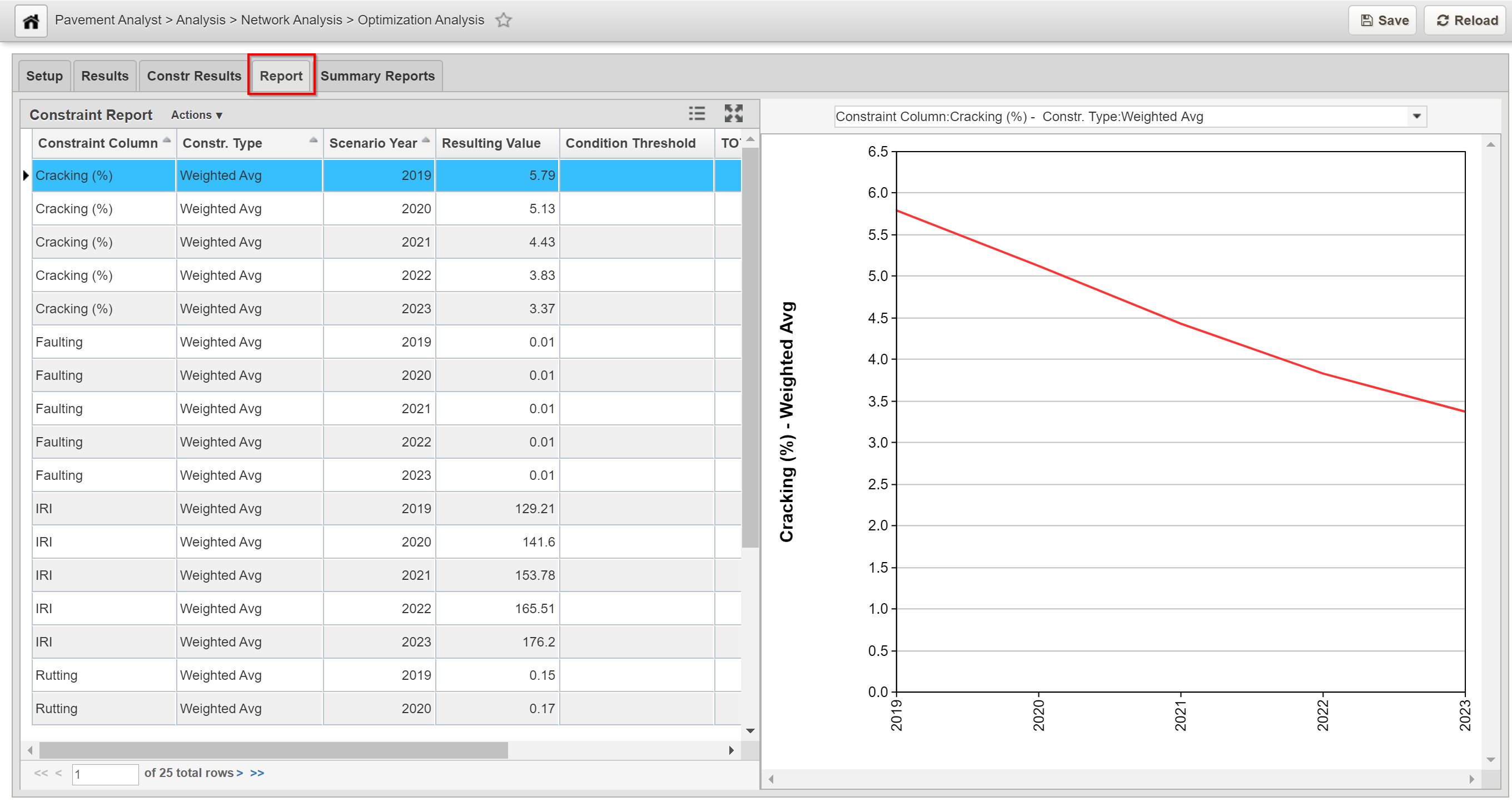
Report Tab

The Report tab shows the constraints you selected in the Reporting Functions pane of the Setup tab and the values of the constraints.

The right pane shows a graph of the values of a particular constraint (which is selected from the drop-down list field shown at the top of the pane). The Y-axis of the graph shows constraint values and the X-axis shows the number of years in the analysis. The graph is a line graph for all constraint types except Total, which is a bar graph. You may modify the appearance of the graph by using the right-click Change Graph Properties commands.

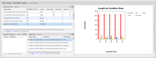
Summary Report Tab

Summary Report window displays the summary graphs of each analysis scenario. These graphs are defined in “Setup Graphs for Summary Report” window and will be the same across all analysis scenarios. The x-axis of each graph is the scenario year, whereas y-axis is defined by an SQL expression. Multiple series can be defined for each graph for comparison purpose among different series. For example, a “Length by Condition State” summary report will display the lane-miles of each condition state for each year, where the scenario year is displayed as the x-axis, the total lane-miles is displayed as the y-axis, and Condition State is displayed as different Series. All these parameters can be configured “Setup Graphs for Summary Report” window.

The left top pane shows each type of summary report, the left bottom pane shows the summary data by each series and scenario year, and the right pane displays the summary graph. You may modify the appearance of the graph by using the right-click Change Graph Properties command.