Finest Partition Report
Finest partition is a method by which you can take data from multiple different tables (i.e., different sets of segmentation) within the system and combine them to produce one output dataset that has homogeneous attributes from across different sets of segmentations. This is done by utilizing the concept of Finest Partition.
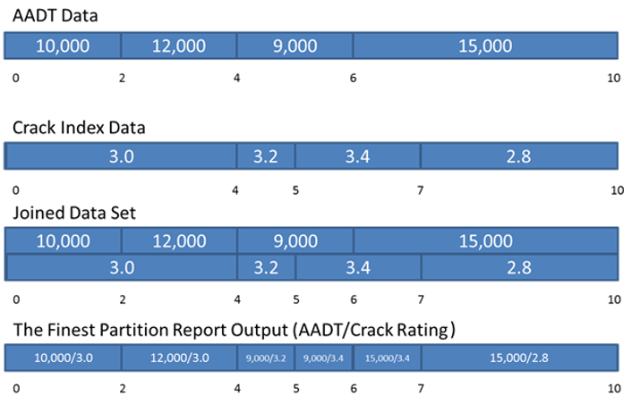
Finest Partition is the smallest set of Linearly Referenced sections that encompass all the lateral and longitudinal breaks across and input data set. This is best illustrated by some simple examples. Suppose we wish to produce a report that combines data from a traffic table listing AADT counts with a table that lists crack index ratings. In the following example, we are combing results from various datasets on a single Route: 999999. The route is 10 miles long.
Traffic data:
Route | Dir | Lane | From | To | AADT |
|---|---|---|---|---|---|
999999 | All | All | 0 | 2 | 10,000 |
999999 | All | All | 2 | 4 | 12,000 |
999999 | All | All | 4 | 6 | 9,000 |
999999 | All | All | 6 | 10 | 15,000 |
Cracking data:
Route | Dir | Lane | From | To | Crack Index |
|---|---|---|---|---|---|
999999 | All | All | 0 | 4 | 3.0 |
999999 | All | All | 4 | 5 | 3.2 |
999999 | All | All | 5 | 7 | 3.4 |
999999 | All | All | 7 | 10 | 2.8 |
The finest partition of these two data sets will create a new table that contains all the section breaks required to fully breakdown both tables. The table below shows the result of the finest partition process on the example data sets. Note that every milepoint from both datasets are present in the resulting data set. This gives a smallest breakdown of the output dataset.
Route | Dir | Lane | From | To | Crack Index | AADT |
|---|---|---|---|---|---|---|
999999 | All | All | 0 | 2 | 3.0 | 10,000 |
999999 | All | All | 2 | 4 | 3.0 | 12,000 |
999999 | All | All | 4 | 5 | 3.2 | 9,000 |
999999 | All | All | 5 | 6 | 3.4 | 9,000 |
999999 | All | All | 6 | 7 | 3.4 | 15,000 |
999999 | All | All | 7 | 10 | 2.8 | 15,000 |
Finest Partition Example:
Point Data
One special case of the finest partition process is dealing with data that is stored as points rather than linear events. Continuing the example above, suppose we add in another point-based data set containing descriptions of specific milepoints within the system.
Route | Dir | Lane | From | To | Description |
|---|---|---|---|---|---|
999999 | All | All | 0 | 0 | Start Route 999999 |
999999 | All | All | 1.5 | 1.5 | Intersection Route 999998 |
999999 | All | All | 2.3 | 2.3 | Driveway Left |
999999 | All | All | 7 | 7 | Entrance Shopping Center |
999999 | All | All | 8.5 | 8.5 | Intersection Route 999997 |
When using point-based data sets, the finest partition process will simply insert breaks into the output dataset wherever the points are located. So, the output from the example included the point events would appear as listed in the table below.
Route | Dir | Lane | From | To | Crack Index | AADT |
|---|---|---|---|---|---|---|
999999 | All | All | 0 | 1.5 | 3.0 | 10,000 |
999999 | All | All | 1.5 | 2 | 3.0 | 10,000 |
999999 | All | All | 2 | 2.3 | 3.0 | 12,000 |
999999 | All | All | 2.3 | 4 | 3.0 | 12,000 |
999999 | All | All | 4 | 5 | 3.2 | 9,000 |
999999 | All | All | 5 | 6 | 3.4 | 9,000 |
999999 | All | All | 6 | 7 | 3.4 | 15,000 |
999999 | All | All | 7 | 8.5 | 2.8 | 15,000 |
999999 | All | All | 8.5 | 10 | 2.8 | 15,000 |
When dealing with point data however the “Description” information must be applied in a different matter since the description only applies to the beginning or ending point of each output data section. Consider the “Driveway Left” description that occurs at milepoint 2.3, it is a valid description for “to” point of the section from 2 through 2.3 and it is a valid description of the “from” point of the section starting at 2.3 through 4. For this reason, we must have 2 output columns in the resulting data set to show the proper point-based data attributes for the from and to locations on each output section.
Route | Dir | Lane | From | To | Crack Index | AADT | From Description | To Description |
|---|---|---|---|---|---|---|---|---|
999999 | All | All | 0 | 1.5 | 3.0 | 10,000 | Start Route 999999 | Intersection Route 999998 |
999999 | All | All | 1.5 | 2 | 3.0 | 10,000 | Intersection Route 999998 | |
999999 | All | All | 2 | 2.3 | 3.0 | 12,000 | Driveway Left | |
999999 | All | All | 2.3 | 4 | 3.0 | 12,000 | Driveway Left | |
999999 | All | All | 4 | 5 | 3.2 | 9,000 | ||
999999 | All | All | 5 | 6 | 3.4 | 9,000 | ||
999999 | All | All | 6 | 7 | 3.4 | 15,000 | Entrance Shopping Center | |
999999 | All | All | 7 | 8.5 | 2.8 | 15,000 | Entrance Shopping Center | Intersection Route 999997 |
999999 | All | All | 8.5 | 10 | 2.8 | 15,000 | Intersection Route 999997 |
Dealing with Directional Data
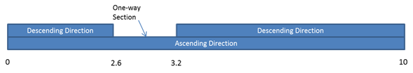
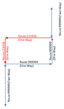
Sometimes the input data sets include data that is directional, which means that the data does not apply to both directions of travel. This is also handled by the finest partitioning process by splitting the incoming data sets into its component directions as well. This requires some more information to be made available about the network. In order to properly split data laterally we must know how many directions are valid within the network at any given point. For example, a route that is two-way its whole length has 2 valid directions at any given point along its length. If a route were one-way its whole length, then it would only have one valid direction at any point. Usually with divided and undivided routes it is possible for a route to contain a mix of two-way and one-way sections along its length. In the following example, Route 999999 has a short portion between miles 2.6 and 3.2 where the route goes through a town and is one side of one-way couplet in town. Therefore, between 2.6 and 3.2 there is only one valid direction, for discussion this direction will be the ascending mile posting direction. Conceptually this might look like following figures.
Information about directionality is stored in a special network definition table within the system called “NETWORK_LINE_DIRECTIONS.” This table contains information about how many directions are valid at any given point along each defined route. For this example the data contained in NETWORK_LINE_DIRECTIONS is as listed in the table below.
Route | Dir | Lane | From | To |
|---|---|---|---|---|
999999 | Asc | All | 0 | 10 |
999999 | Desc | All | 0 | 2.6 |
999999 | Desc | All | 3.2 | 10 |
The data structure contains only information where a particular direction is valid. In this case the Ascending Direction is valid for the whole length on the route, but the descending direction is only valid for the milepoint ranges 0 to 2.6 and 3.2 to 10.
To expand the example Finest Partition, we will add in another table with Pavement Type Information that is stored on a directional basis, as in the table below.
Route | Dir | Lane | From | To | Pavement Type |
|---|---|---|---|---|---|
999999 | Asc | All | 0 | 4 | AC |
999999 | All | All | 4 | 5 | AC |
999999 | All | All | 5 | 7 | PCC |
999999 | All | All | 7 | 10 | PCC |
999999 | Desc | All | 0 | 2 | Composite |
999999 | Desc | All | 3.5 | 4 | Composite |
The addition of directional data into the finest partitioning process introduces some extra complexity that should be understood in setting up a Finest Partition report. To begin the system will start by looking at all unique breaks from the source data within a route and then looking at how many distinct directions exist in the source data within each of those sections, as shown in the table below.
| Route | From | To | Number of Directions in Source Data |
|---|---|---|---|
| 999999 | 0 | 1.5 | 3 (All, Asc, Desc) |
| 999999 | 1.5 | 2 | 3 (All, Asc, Desc) |
| 999999 | 2 | 2.3 | 2 (All, Asc) |
| 999999 | 2.3 | 3.5 | 2 (All, Asc) |
| 999999 | 3.5 | 4 | 3(All, Asc, Desc) |
| 999999 | 4 | 5 | 1 (All) |
| 999999 | 5 | 6 | 1 (All) |
| 999999 | 6 | 7 | 1 (All) |
| 999999 | 7 | 8.5 | 1 (All) |
| 999999 | 8.5 | 10 | 1 (All) |
Sections in the table above that have only 1 distinct direction in the source data may be moved directly into the final output of the process as no further partitioning is required. In this example all the sections starting at mile 4 or higher only have one direction defined across all the source data. These are put immediately into the output table, shown in the table below leaving only the miles from 0 to 4 to be processed further.
Route | Dir | Lane | From | To | Crack Index | AADT | Pavement Type | From Description | To Description |
|---|---|---|---|---|---|---|---|---|---|
999999 | All | All | 4 | 5 | |||||
999999 | All | All | 5 | 6 | |||||
999999 | All | All | 6 | 7 | |||||
999999 | All | All | 7 | 8.5 | |||||
999999 | All | All | 8.5 | 10 |
The next step in the process is to consider breaks on each direction individually. This is a 4-step process:
- Start with the remaining contiguous sections of the road in the direction of interest (no breaks within each contiguous section).
- Add in any breaks for that direction listed in the NETWORK_LINE_DIRECTIONS table. If the source data has (All) Direction, it will also remove any portions not covered within NETWORK_LINE_DIRECTIONS.
- Add in any additional breaks from the source data
- Copy the resulting sections into the output with the Direction field set to the direction of interest.
- Go back to step one for any additional directions of interest
The resulting data set may then be copied into the output. For this example, we will consider first the “Asc” direction. So we start with the remaining portion of the route mile 0 to mile 4. Then we add in any breaks within the 0 to 4 milepoint range from the NETWORK_LINE_DIRECTIONS table. Since NETWORK_LINE_DIRECTIONS has only 1 section covering 0 to 10 there are no extra breaks required and that leaves only 1 section from 0 to 4. Next we apply any additional breaks on the “Asc” direction contained in the source data. Applying these breaks from the source data to the 0 to 4 section gives use the sections listed below:
Route | Dir | Lane | From | To | Crack Index | AADT | Pavement Type | From Description | To Description |
|---|---|---|---|---|---|---|---|---|---|
999999 | Asc | All | 0 | 1.5 | |||||
999999 | Asc | All | 1.5 | 2 | |||||
999999 | Asc | All | 2 | 2.3 | |||||
999999 | Asc | All | 2.3 | 4 |
Continuing with the Descending direction in the same manner gives the following output:
Route | Dir | Lane | From | To | Crack Index | AADT | Pavement Type | From Description | To Description |
|---|---|---|---|---|---|---|---|---|---|
999999 | Desc | All | 0 | 1.5 | |||||
999999 | Desc | All | 1.5 | 2 | |||||
999999 | Desc | All | 2 | 2.3 | |||||
999999 | Desc | All | 2.3 | 2.6 | |||||
999999 | Desc | All | 3.2 | 3.5 | |||||
999999 | Desc | All | 3.5 | 4 |
Note that on the descending direction there is a “hole” in the data between 2.6 and 3.2 because the NETWORK_LINE_DIRECTIONS table does not cover that portion of the route in the Desc direction.
The table below shows the results of the finest partitions together (from the three previous tables) with attribute information from the source data. For clarity we have sorted the table below by “From” and ”Direction.”
Route | Dir | Lane | From | To | Crack Index | AADT | Pavement Type | From Description | To Description |
|---|---|---|---|---|---|---|---|---|---|
999999 | Asc | All | 0 | 1.5 | 3.0 | 10,000 | AC | Start Route 999999 | Intersection Route 999998 |
999999 | Desc | All | 0 | 1.5 | 3.0 | 10,000 | Composite | Start Route 999999 | Intersection Route 999998 |
999999 | Asc | All | 1.5 | 2 | 3.0 | 10,000 | AC | Intersection Route 999998 | |
999999 | Desc | All | 1.5 | 2 | 3.0 | 10,000 | Composite | Intersection Route 999998 | |
999999 | Asc | All | 2 | 2.3 | 3.0 | 12,000 | AC | Driveway Left | |
999999 | Desc | All | 2 | 2.3 | 3.0 | 12,000 | NULL | Driveway Left | |
999999 | Asc | All | 2.3 | 4 | 3.0 | 12,000 | AC | Driveway Left | |
999999 | Desc | All | 2.3 | 2.6 | 3.0 | 12,000 | NULL | Driveway Left | |
999999 | Desc | All | 3.2 | 3.5 | 3.0 | 12,000 | NULL | ||
999999 | Desc | All | 3.5 | 4 | 3.0 | 12,000 | Composite | ||
999999 | All | All | 4 | 5 | 3.2 | 9,000 | AC | ||
999999 | All | All | 5 | 6 | 3.4 | 9,000 | PCC | ||
999999 | All | All | 6 | 7 | 3.4 | 15,000 | PCC | Entrance Shopping Center | |
999999 | All | All | 7 | 8.5 | 2.8 | 15,000 | Composite | Entrance Shopping Center | Intersection Route 999997 |
999999 | All | All | 8.5 | 10 | 2.8 | 15,000 | Composite | Intersection Route 999997 |
Finest Partition System Executable
Finest Partition system job executable allows the user to use one or multiple tables as the input and execute Finest Partition process as described in the last section, and save the results into another target table (Finest Partition Report does not save the results into any table - it's a report). Finest Partition executable only produces the resulted segment, and does not populate any attributes. Normally user will configure the result table to include any desired attributes (columns), configure Update Target Table SQL, and executable Update Target Table command or executable to populate these columns.
There are two system Finest Parition executables: Finest Partition and Finest Partition by Column. The difference is explained in the following section.
To create and execute Finest Partition System Job, follow these steps:
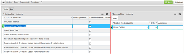
- Go to the System Schedules window, located under System > Tools > System Job > Schedules
- In the Schedules pane (left pane), insert a new system job schedule and give it a name. Then in the Executables pane (right pane), insert Finest Partition executable or Finest Partition by Column executable.
- Right-click the executable and select Define Argument(s)
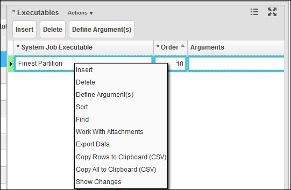
- Right click the executable and select “Define Argument(s)”.
- If “Finest Partition” executable is used, a pop-up window shows up with 3 fields:
Input SQL Statement – This is an SQL query that returns all sections to be Finest Partitioned with their corresponding ROUTE_ID, LANE_ID, LANE_DIR, OFFSET_FROM and OFFSET_TO from SETUP_LOC_IDENT table. When there are multiple tables as input, a “UNION” keyword can be used to combine them. Below is an example that performance Finest Partition between PMS_ROADWAY_INVENTORY and PMS_MGMT_SECTIONS table:
SELECT LA.ROUTE_ID, LA.LANE_ID, LA.LANE_DIR, LA.OFFSET_FROM, LA.OFFSET_TO
FROM PMS_ROADWAY_INVENTORY A, SETUP_LOC_IDENT LA
WHERE A.LOC_IDENT = LA.LOC_IDENT AND LA.SOURSE_TABLE = ‘PMS_ROADWAY_INVENTORY’
UNION
SELECT LA.ROUTE_ID, LA.LANE_ID, LA.LANE_DIR, LA.OFFSET_FROM, LA.OFFSET_TO
FROM PMS_MGMT_SECTIONS A, SETUP_LOC_IDENT LA
WHERE A.LOC_IDENT = LA.LOC_IDENT AND LA.SOURSE_TABLE = ‘PMS_MGMT_SECTIONS’
Note: Overlapping sections or duplicating sections are permitted in this Input SQL Statement. Finest Partition job will process them accordingly and output the results based on the principles defined in the last section.
- Target Table Name – This the table where the result segments from Finest Partition will be saved. This table must be a strictly Location-referenced data table (see detailed discussion in AgileAssets System Foundation Configuration Guide, or this link on docs.agileassets.com)
- Delete Where Clause – This is an optional where clause that can be applied to Target Table. All records in the target table that match the where clause will be deleted when running the Finest Partition executable. If left empty, all records in the target table will be deleted
- If Finest Partition by Column executable is used, a pop-up window shows up with 4 fields:
Input SQL Statement – This is an SQL query that returns all sections to be Finest Partitioned with their corresponding ROUTE_ID, LANE_ID, LANE_DIR, OFFSET_FROM and OFFSET_TO from SETUP_LOC_IDENT table. This argument is the same as the other executable.
Target Table Name – This the table where the result segments from Finest Partition will be saved. This argument is the same as the other executable.
Column ID and Column Value Setup – When the executable is used, the system will first delete the records from the Target Table that match the Column ID argument and Column Value argument, then, after the Finest Partition output is saved to the Target Table, it will also fill Column ID with the Column value.
Note: This function supports only one column.
Output of Finest Partition executable only includes the section definitions and will not automatically calculate the attributes (i.e., any columns other than LOC_IDENT column in Target Table Name argument, or the Column ID column when using the “Finest Partition by Column” executable). Therefore, the Finest Partition executable is typically followed by an “Update Target Table” executable, which fills in all attribute values in the target table.
NOTE: To be able to use Update Target Table, the data aggregation SQL statement must be defined on the corresponding columns in the table.
- Right-click and new System Schedule and select Run Job to run the Finest Partition job.